Not only is this feature useful to you as the spreadsheet editor, it’s also helpful to people that are going to be reading the data on their own computer screen.
Microsoft Excel Lock Row Steps
You can continue below for more information on the Excel lock row process, including how to freeze multiple rows, as well as how to unfreeze a row or rows that you have previously frozen. Learning how to lock rows in Excel is a great way to ensure that your important information, such as your column headings or titles, remain visible. Large spreadsheets can be difficult to manage in Microsoft Excel 2013, whether they are being printed or shown on the screen. Another useful step to take when trying to view data is learning how to expand all rows in Excel so that you can see all of your information. One of the most troubling parts of editing a large spreadsheet is making sure that data you enter is being placed into the correct column. This can lead to a lot of scrolling up and down through the worksheet as you check your column headings to make sure you are entering data into the correct cell. One way to simplify this process is to freeze some rows in your spreadsheet. That way they remain visible at the top of your worksheet while you scroll down to the rows that you are editing. Our tutorial below will show you how to freeze and unfreeze rows in your worksheet. Find out how to autofit all columns in Excel if you want a fast way to make all of your cell data visible.
How to Freeze One or More Rows in an Excel 2013 Spreadsheet (Guide with Pictures)
The steps in this article were performed in Microsoft Excel 2013, but will also work in other Excel products that use the ribbon navigation system, such as Excel 2007 and Excel 2010.
Step 1: Open your spreadsheet in Excel 2013.
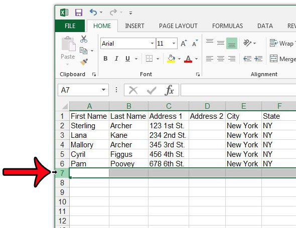
Step 2: Click the row below the rows that you want to freeze.
I am clicking row 7 in the picture below, as I want to freeze the top 6 rows.
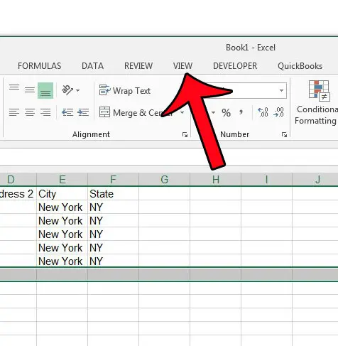
Step 3: Click the View tab at the top of the window.
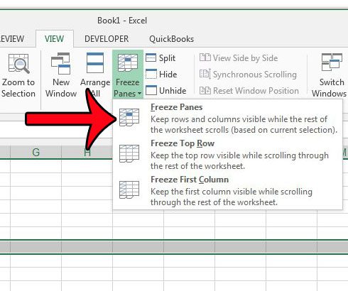
Step 4: Click the Freeze Panes button in the Window section of the ribbon, then click the Freeze Panes button.
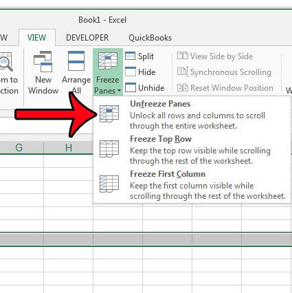
Note that you also have the choice of clicking the Freeze Top Row option as well, if you are only looking to freeze the first row of your worksheet. You can now scroll down your spreadsheet to view additional rows, while the frozen rows will remain visible at the top of the sheet. Now that you are familiar with the Excel lock row process, it’s helpful to know how to unlock rows that you have frozen as well. Once you have finished with the need to have the rows frozen, you can click the Freeze Panes button again, then click the Unfreeze Panes button.
How to Unfreeze a Row in Excel
The method for unfreezing rows in Excel is very similar to how we were able to freeze a row in the guide above. This will remove any frozen panes in the worksheet, allowing you to work without them, or to elect to freeze a different row or rows in Excel. You can use a similar method to the one described in this article to freeze the top row of an Excel spreadsheet. This is helpful if you are using a common Excel layout that uses the first row of the worksheet to label the data that will appear in the columns underneath it. Additionally, if you need to print your spreadsheet, then you can also print the top row on every page so that your readers won’t get lost as they read pages beyond the first one of the spreadsheet.
Additional Sources
After receiving his Bachelor’s and Master’s degrees in Computer Science he spent several years working in IT management for small businesses. However, he now works full time writing content online and creating websites. His main writing topics include iPhones, Microsoft Office, Google Apps, Android, and Photoshop, but he has also written about many other tech topics as well. Read his full bio here.
You may opt out at any time. Read our Privacy Policy


